Kaggle Ultrasound Nerve Segmentation (25th with 0.70679 final ranking)
19 Aug 2016 | Programming
I participated in the Ultrasound Nerve Segmentation Kaggle challenge and it looks like my final rank is 25th (I was 48th on the public leaderboard).
The github repo with my code is available here. I should warn you that since this was a 3 months competition, the code is not optimized for reuse and probably quite messy with a lot of copy-paste.
1. Data
The goal of the competition was to label the area containing a collection of
nerves called the Brachial plexus in ultrasound images. So the model is given an grayscale image
as input and should output a binary image (= a binary mask). Some images (about 60% of the training set) do not contain the Brachial plexus area and should
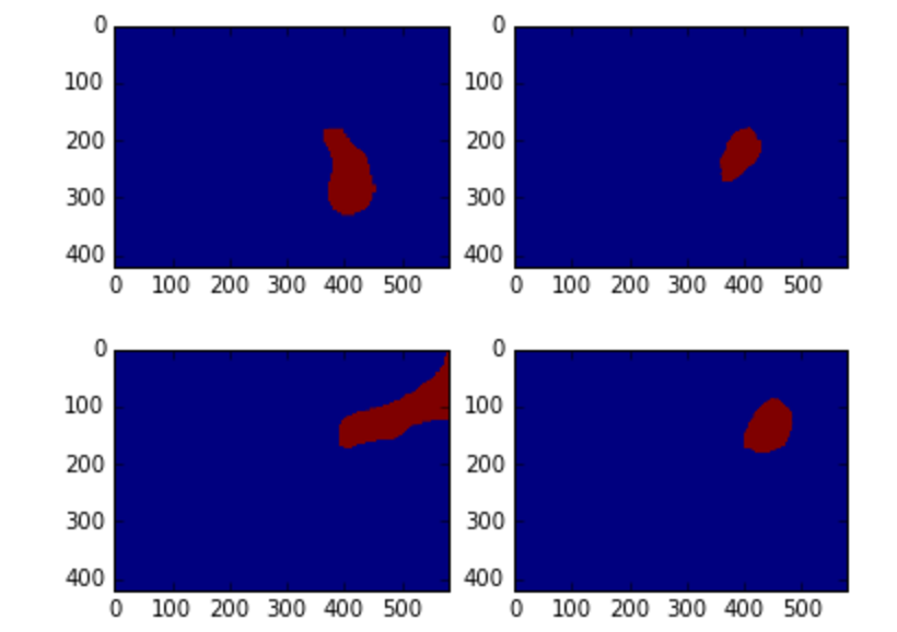
therefore have an empty mask. It basically looks like this :
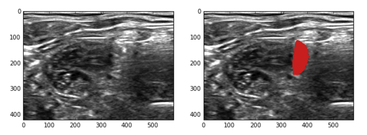
(left is the image, right is the image and the label area overlayed in red)
You can have also a look at this script on kaggle which has a nice animation of some of the images.
The images have a size of 580x420 pixels. There are 5635 training images and 5508 test images (of which 20% were used for public ranking and 80% for the final ranking).
Contradictory labelling in the training data
As many people found out during the competition, the training dataset contains many contradictory examples. By contradictory examples, I mean two images that are very similar but with one image having a non-empty mask and the other one having an empty mask.
Here is an example. The top image has no mask while the one at the bottom has one.
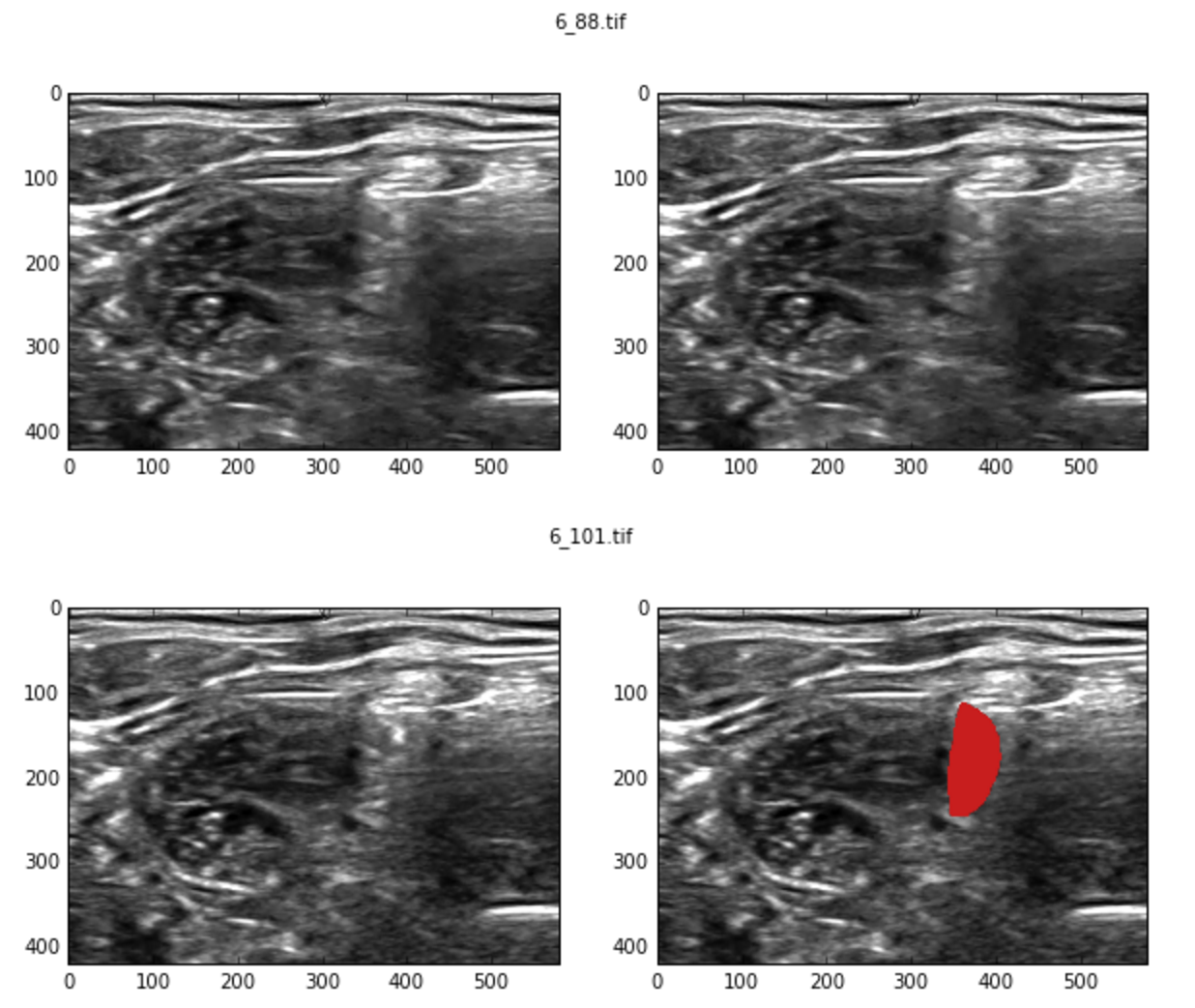
There are a huge number of similar examples in the training set and this puts a (somewhat low) upper bound on the best result you can achieve, regardless of the model.
I believe the problem is partly due to the fact that the images are actually video frames. So the human expert who is putting the label does so using the video. But the challenge was set up in a way that we had to labellize individual images and they shuffled the frames to force us to NOT rely on the temporal information. I wonder why this choice was made since having videos instead of images could have been very interesting (CNN-RNN !).
2. Model and results
This is an image segmentation problem. Like many people in the challenge, I decided to use some deep learning as it works so well on images. I tried multiple architectures, but they are all based on fully-connected CNN or U-net.
Before talking about model, here is the evolution of my score on the public LB.
As you can see, I had a pretty solid start and then spent much time trying to
get really small incremental improvements (the red line indicates my best).
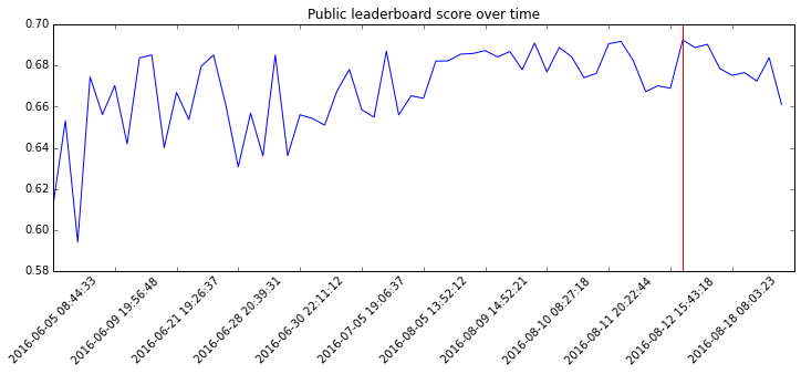
The subnotes.txt file in my repo contains some notes about each submission so I could keep track of what was helpful or not.
Pre-processing
Image scaling
The images have a size of 580x420. This is quite big and when I first tried to train a CNN (using a GTX 960) on those images, I quickly ran into memory and performance problems.
Also, since I wanted to do a fully-connected network, it’s much easier if the size of the image is a power of two, so you can pool and unpool without having to fiddle with padding.
I quickly decided to rescale my images to 128x128. I don’t have much data to back that claim, but this helped me train my networks much faster without loosing predictive power. This also mean I stretched the images (the scale factor isn’t the same for both axes), but this didn’t seem to hinder performances much.
Removing contradictory images
Based on what I highlighted above about contradictory labelling in the training set, I decided to remove the training images without a mask that were close to another training image with a mask.
I computed the similary between two images by computing a signature for each image as follow : I divided the image in small 20x20 blocks and then compute a histogram of intensity in each block. All the histograms for the image are then concatenated into a big vector. The disimilary is the the cosine distance between the two signature vectors of two images. This is what is done in the 13_clean/0_filter_incoherent_images.ipynb notebook.
This results in a distance matrix for all the training set images, which is then thresholded to decide which images should be removed. In the end, I kept 3906 training images (out of the 5500).
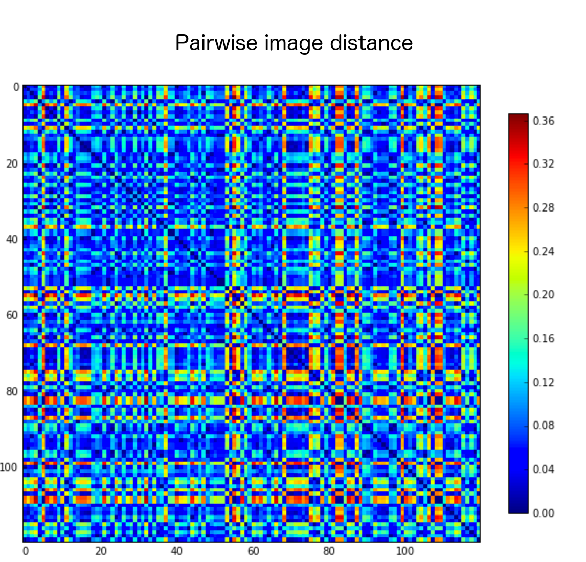
I also tried propagating masks instead of removing images, but this didn’t seem to help.
Architecture
My best single-model submission is from this notebook. It scored 0.69167 on the public LB nad 0.69234 on the private.
This is a multiple objective model as you can see in the following diagram :
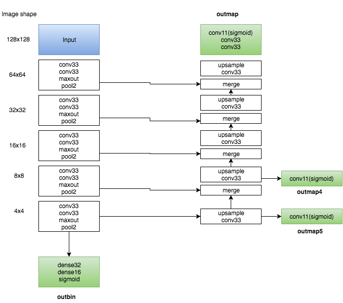
The left part is a traditional CNN. After all the convolutions + pooling, there is a small dense network that has a single output (called outbin) which is the probability that the image has a non-empty mask.
The right part is similar to the U-net where we upsample and merge at each level.
The real output is the outmap one (the top green box) which contains the predicted mask.
In addition, I added two auxiliary outputs (outmap4 and outmap5) which are trained to predict very coarse (4x4 and 8x8) masks. This is only used for training and it looked like it helped a bit regularize the training.
I also found that using Maxout activations seemed to help the training a bit. I am not sure if I could have achieved the same perf by just increasing the number of epochs or by fine-tuning the learning rate.
This model has 95000 parameters. I found difficult to train models with more parameters without overfitting and I got really good results with 50000 parameter models as well.
I used some very simple data augmentation (small rotation, zoom, shear and translation). From some posts on the forum, it looks like doing some horizontal flips helped a lot, but I (wrongly apparently) thought that was a bad idea because the masks are not symmetric and so I didn’t explore that.
My best submission (0.70679 private LB)
This was submission 54 which scored 0.69237 on the public LB. This is an ensemble of the 4 models which got the best public LB scores. The ensembling is done in this notebook.
Post-processing
Sometimes, the predicted mask has some “holes” or incoherent shape. I tried three different post-processing approaches :
- Morphological close to remove small holes. This helped a bit
- Fitting an ellipse to the mask and filling the ellipse (since the mask are often somewhat ellipse-like). This didn't help and even sometimes decreased the performance.
- Using a PCA decomposition of the training masks and reconstruct the predicted mask using a limited number of principal components. This seemed to help more consistently (although just a little bit).
PCA cleaning
The idea of using PCA to post-process came from the Eigenface concept. Basically, you consider your image as a big vector and you then do PCA on the training masks to learn “eigenmasks”.
To clean a predicted mask using this method, you project the cleaned mask on the subspace found by PCA and you then reconstruct using only the 20 (in my case) first principal components. This forces the reconstructed mask to have a shape similar to the training masks.
Here are two extreme examples (predicted mask is left, PCA-cleaned is right) :
Loss and mask percentage
I tried using dice coefficient as a loss, but I always got better results by using binary cross-entropy.
An empty submission on the public leaderboard gets a score of 0.51. This means 51% of the images have no mask. So 49% of the images should have mask and I tried to optimize the threshold on the binary and mask output to get close to 49% predicted masks. But in the end, my best submissions have around 35%-38% of predicted masks. I guess this is because lowering the thresholds to get higher number of predicted masks leads to too many false positive.
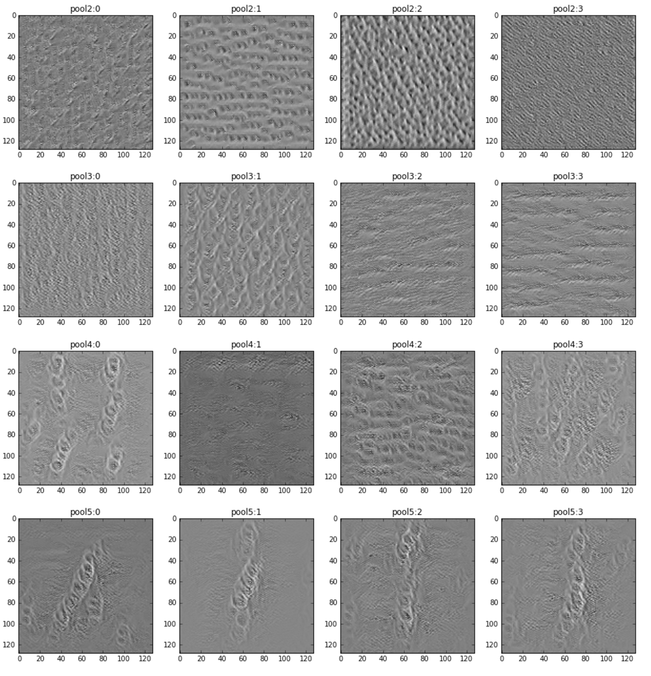
3. Dreaming nerves
Once you have a trained CNN, you can make the network “dream” to visualize what the networks wants to see to maximize some output or some intermediate layer. This gives a pretty picture that’s also useful for debugging.
In the image below, you can see some example input images that maximizes the activation of specific filters (each row has 4 filters of a given depth).
The fourth row is the innermost convolutional layer and you can clearly see that the network reacts to interleaved nerve structure.
4. Conclusion
This was an interesting competition. I learnt a lot by playing with various architectures and trying various pre/post-processing techniques.
One problem was the dataset labelling quality. Although it is a good challenge (and something common in everyday applications) to deal with contradictory or inconsistent labels, I think it hurts the competition because people spend time trying to predict the labelling mistakes instead of trying to build a better model of the problem.